Thousands of animals are present in shelter homes and much more are present on the
streets. In order to stop things like cruelty and euthanization of these animals, we
need to increase animal adoption rates. Animals with cute pictures are more likely to
get adopted. Shelters need a way to estimate and increase “cuteness” of
photos of these animals to get them adobted faster. The goal of our project is to use
machine learning to make accurate predictions of “cuteness” and increase animal adoption
rates from the shelters.
Problem definition
For CS7641, our project aims at estimating the cuteness/popularity of images of shelter animals.
This is an open kaggle
challenge.
The dataset contains raw images of shelter animals along with metadata.
The metadata consists of a set of binary features like presence of eyes, face, etc.
In this project, we use both supervised learning and unsupervised learning to estimate
popularity/cuteness of images. In particular, we use representation learning to learn features
from raw images along with PCA to select prominent features from the metadata. Finally, we plan
on demonstrating the effectiveness of our solution by plotting training and validation loss
along with an ablation study.
Dataset Description
Metadata Description:
For each image in the trainng set, we also have a set of metadata available. The metadata contains
information regarding the following binary feature:
Focus, Eyes, Face, Near, Action, Accessory, Group, Collage, Human, Occlusion, Info, Blur
Image data details:
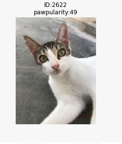
We have a training data set of close to\(10,000\) RGB images.
Each image has a pawpularity score as shown in [Fig 1]
[Fig 1] Example image data available in the dataset
Metadata exploration
Linear Regression on Metadata
The metadata was split into a 80-20 share for the purposes of training and testing the data. All data reported are for
the test set.
Without PCA:
We first ran Linear Regression on the metadata. However, the \(R^2\) score of the regressor turned out to be very poor at
only \(0.003\). This meant that the variation in the input features did not explain the variation in target. Additionally,
the RMSE score was \(20.4944\).
With PCA [Unsupervised Learning]:
We next ran PCA on the meta-data with an intention to retain \(90%\) of the variance in data. We then again ran the
transformed features against the target variables. This reduced the \(R^2\) of the model to an even lower value of \(0.0001\).
We also used lightgbm on the metadata to check if introduction of non-linearilty helps in the regression.
However, the rmse score stayed at \(~20\). The best RMSE score we were able to achieve using lightgbm was \(20.466760\)
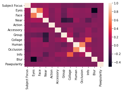
The outputs of the Linear Regressor made us question the quality of the data and its relation to the target variable.
Therefore, we quickly checked the correlation of the input features with the target data. The results indicated that the
metadata contained practically zero correlation with the metadata as can be seen in the [Fig 2] and
there is not much information value in the metadata. [Fig 2] Correlation Matrix
Image exploration
Image data exploration
While manually inspecting the data we found that the dataset has a lot of noise.
Individually looking at the photos, we noticed that the popularity score did not always tally
with the cuteness/quality of the animal. In addition to this, we also noticed that there are several
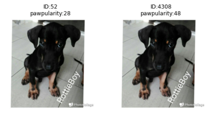
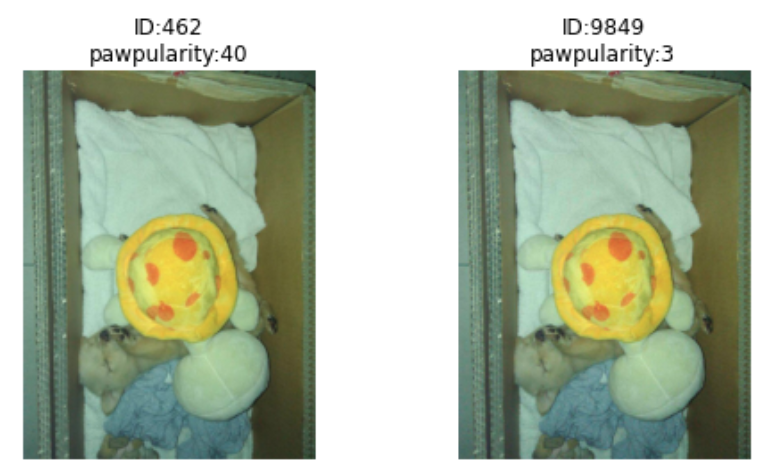
duplicate images with different popularity scores in the dataset.
Given this new found knowledge, we tried multiple ways to wrote a small script to extract the
duplicate images by cosine similarity between the pairs of images. We chose to flatten the image and then
found the similarity between two images using the formula: \(a.b / |a||b|\)
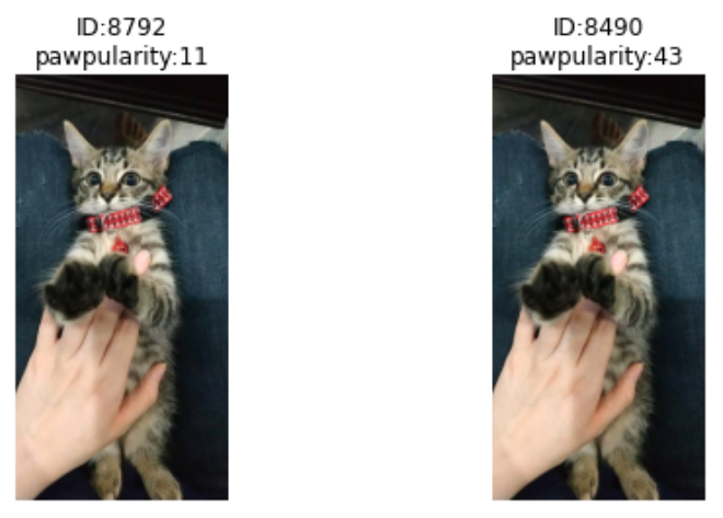
The images below show a sample of the duplicate images with contradictory pawpularity scores that we were able
to find.
[Fig 3] Some examples of duplicate images With this information we chose to exclude these images from our training and test set.
Supervised CNN model finetuning
We convert all the RBG images \((0,255)\) to pytorch tenors with values scaled to \((0,1)\)
Input images have different sizes and we resize them to \(256\times256\)
Then we normalize all the images with a mean of \((0.485, 0.456, 0.406)\) and std of \((0.229, 0.224, 0.225)\) which are
determined to give better performance on imagenet models like resnet18 etc based on the imagenet image
statistics
We used deep neural networks to perform regression on the image data.
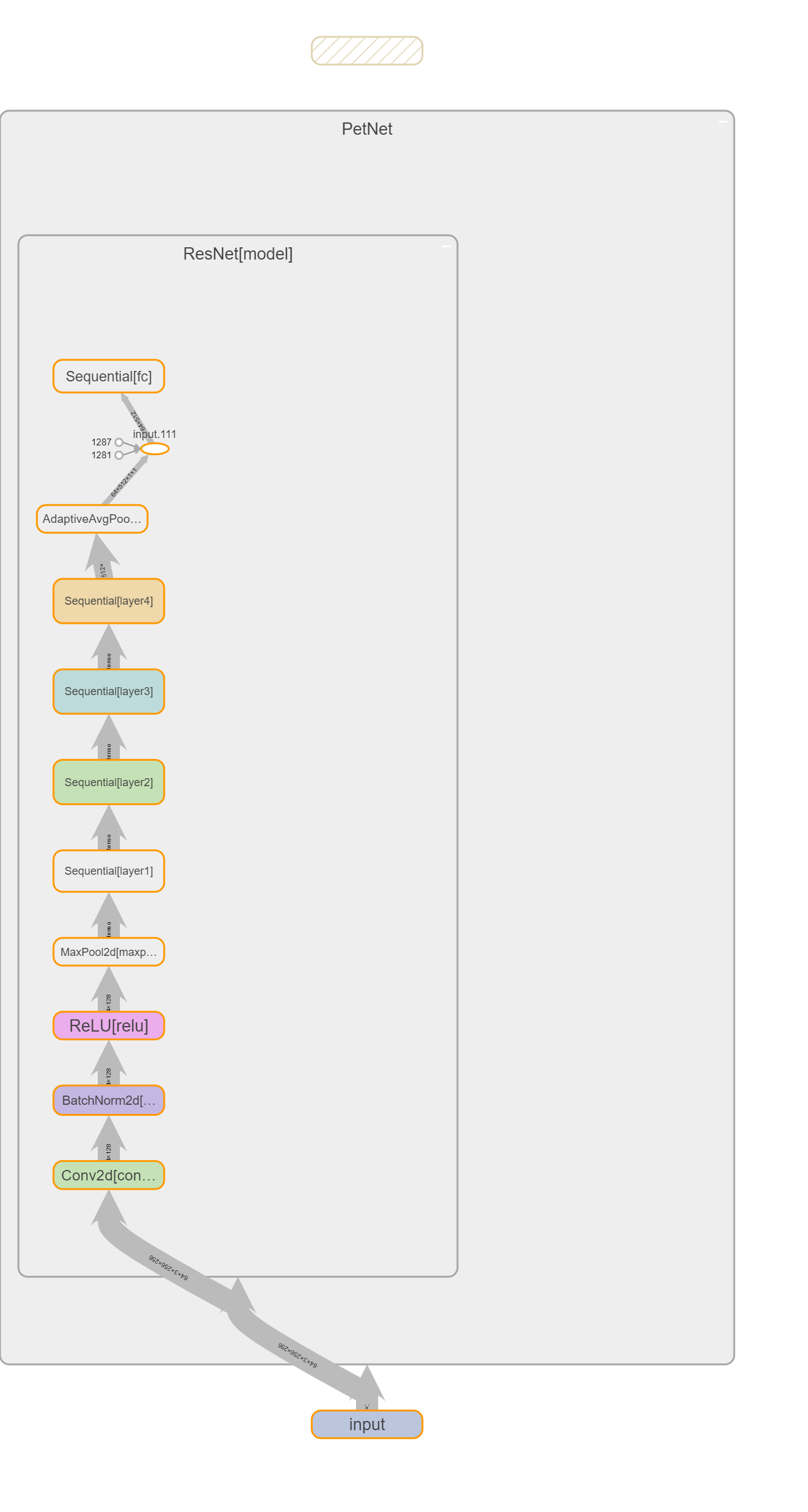
The final modelstructure is as below:
resnet18 as the fixed image feature extractor
multi-layer fully connected network as the regressor head
Below is a figure of the model: [Fig 4] Model architecture
We ran the model against the target pawpularity score. This provided us an RMSE score of \(19.187\)
Below is the plot of RMSE loss in terms of epoch. As we can see the from the training loss plot, we are able to reduce the RMSE from \(40\) to \(20\) using the above deep
architecture.
[Fig 5] Training loss change with epochs
Final validation RMSE turns out to be \(19.18\) which means there is not much of performance boost from the deep neural
model. This might be because of the noise in the data and the issue needs further investigation.